Getting Started
This page assumes that you have already installed the pypfilt package, and shows how to generate forecasts for the following system:
Parameters
Particle filter parameters are provided by default_params().
Observation model parameters (and fixed parameters for the process model, if any) should be added to this parameter dictionary, so that all parameters pertaining to the simulation are stored together.
def get_params(regularisation=False):
    """
    The default simulation parameters.

    :param regularisation: Whether to use the post-regularisation particle
        filter (post-RPF).
    """
    # The particle filter parameters.
    params = pypfilt.default_params(Model, px_count=1000)
    # Provide an observation model.
    params['log_llhd_fn'] = log_llhd
    # System model parameters.
    if regularisation:
        # No need to add stochastic noise to the model equations.
        params['sys'] = {'noise_alpha': 0, 'noise_dx': 0}
    else:
        # Need to add some stochastic noise to the model equations.
        params['sys'] = {'noise_alpha': 5e-3, 'noise_dx': 0.025}
    # Observation model parameters.
    params['obs'] = {'sdev': 0.05}
    # Set a fixed PRNG seed.
    params['resample']['prng_seed'] = 42
    # Define whether to use the post-regularised particle filter.
    params['resample']['regularisation'] = regularisation
    return params
Observations
Observations are represented as dictionaries that have the following keys:
{'date': datetime.datetime(...),  # When the observation was made
 'value': 200,  # The numerical quantity that was measured
 'unit': 'Some measure',  # A description of the measurement units
 'period': 7,  # The observation period, in days
 'source': 'Some system',  # A description of the data source
}
An observation stream is represented as a chronologically sorted list of
observations (oldest first).
The particle filter accepts any number of observation streams, which must be
provided as a list (i.e., a list of observation lists); see
forecast() and run().
Observations can be read from external files:
def obs_from_file(filename, year):
    """
    Read observations from a file with the following format:

    year date       value
    2009 2009-01-02 0.680762021741
    2009 2009-01-03 0.62923826359
    2009 2009-01-04 0.621926239641
    2009 2009-01-05 0.618802422847
    ...
    """
    col_types = [('year', np.int32), ('date', '|O4'), ('value', np.float32)]
    col_types = pypfilt.summary.dtype_names_to_str(col_types)
    col_convs = {1: lambda s: datetime.datetime.strptime(s, '%Y-%m-%d')}
    with codecs.open(filename, encoding='ascii') as f:
        df = np.loadtxt(f, skiprows=1, dtype=col_types, converters=col_convs)
    df = df[df['year'] == year]
    nrows = df.shape[0]
    # Note that counts are assumed to be reported daily (period = 1).
    return [{'date': df['date'][i],
             'value': df['value'][i],
             'unit': 'x',
             'period': 1,
             'source': 'file: {}'.format(filename)}
            for i in range(nrows)]
They can also be generated synthetically:
def generate_obs(x0, alpha, sdev, start, days, seed=42):
    """Generate noisy observations from a known truth."""
    rng = np.random.RandomState(seed)
    time = np.array(range(1, days + 1))
    # Here, x(t) = x(0) * e^{- alpha * t} + error
    xs = x0 * np.exp(- alpha * time)
    if sdev > 0:
        xs += rng.normal(scale=sdev, size=days)
    return [{'date': start + datetime.timedelta(days=i + 1),
             'value': xs[i], 'unit': 'x', 'period': 1,
             'source': 'synthetic'}
            for i in range(days)]
System models
The model of the underlying system must inherit from
pypfilt.model.Base.
Here is a simulation model for the example system:
class Model(pypfilt.model.Base):
    """
    A model of the following system:

        dx/dt = - alpha . x

    The state vector is ``[x(t), alpha]``.
    """

    @staticmethod
    def state_size():
        """Return the length of a single state vector."""
        return 2

    @staticmethod
    def priors(params):
        """Return a dictionary of model parameter priors."""
        a_min, a_max = params['param_min'][0], params['param_max'][0]
        return {
            'alpha': lambda r, size=None: r.uniform(a_min, a_max, size=size),
        }

    @staticmethod
    def init(params, vec):
        """Initialise any number of state vectors."""
        rnd = params['resample']['rnd']
        rnd_size = vec[..., 0].shape
        # Assume that x(0) is somewhere between 0.5 and 1.
        vec[..., 0] = rnd.uniform(0.5, 1.0, size=rnd_size)
        # Select alpha according to the prior.
        vec[..., 1] = params['prior']['alpha'](rnd, size=rnd_size)

    @staticmethod
    def update(params, step_date, dt, is_fs, prev, curr):
        """Perform a single time-step for any number of state vectors."""
        rnd = params['resample']['rnd']
        rnd_size = curr[..., 0].shape
        # Calculate the deterministic change for x.
        dx = prev[..., 0] * prev[..., 1] * dt
        # Add stochastic noise to the rate.
        noise = params['sys']['noise_dx']
        noise *= rnd.normal(size=rnd_size) * dt
        dx += noise * np.sqrt(dx / dt)
        # Add stochastic noise to alpha.
        noise_alpha = params['sys']['noise_alpha']
        noise_alpha *= rnd.normal(size=rnd_size) * dt
        # Update the state vectors, ensuring alpha remains strictly positive.
        curr[..., 0] = prev[..., 0] - dx
        curr[..., 1] = np.clip(prev[..., 1] + noise_alpha,
                               params['param_min'][0], params['param_max'][0])

    @classmethod
    def state_info(cls):
        """Describe each state variable."""
        return [("x", 0)]

    @classmethod
    def param_info(cls):
        """Describe each model parameter."""
        return [("alpha", 1)]

    @classmethod
    def param_bounds(cls):
        """Return the (default) lower and upper parameter bounds."""
        return ([0.01], [0.10])

    @classmethod
    def stat_info(cls):
        """Describe each statistic that can be calculated by this model."""
        return []
Observation models
The observation model must be stored in params['log_llhd_fn'] and have the
following form:
def log_llhd(params, obs_list, curr, prev_dict):
    """
    Calculate the log-likelihood of obtaining specific observations from each
    particle.
    """
    log_llhd = np.zeros(curr.shape[:-1])
    # The expected observation is x(t).
    exp = curr[..., 0]
    # The standard deviation of the observation error.
    sdev = params['obs']['sdev']
    # The likelihood distribution for each particle.
    obs_dist = scipy.stats.norm(loc=exp, scale=sdev)
    for o in obs_list:
        # Calculate the likelihood of this observation for each particle.
        log_llhd += obs_dist.logpdf(o['value'])
    return log_llhd
While the argument prev_dict was not used in this example, it can be used
to obtain the state vectors at the beginning of an observation period:
def log_llhd(params, obs_list, curr, prev_dict):
    # Obtain the state vectors for one week prior.
    # This is only valid if an observation has a period of 7.
    one_week_ago = prev_dict[7]
    dx = curr[..., 0] - one_week_ago[..., 0]
    ...
This is useful for situations where the observation depends on the change in the state vector over the observation period.
Summary objects
Simulations typically comprise a large number of both particles and time steps, and so it is generally preferable to record statistics that summarise the particles than to store the entire state history of each simulation.
This functionality is provided by pypfilt.summary.HDF5, which allows
any number of summary tables to be recorded. Once all of the estimation and
forecasting simulations have been performed,
save_forecasts() will save the results to disk.
Here is an example of how to record fixed-probability central credible
intervals for the state variable \(x\) and model parameter \(\alpha\)
of the example system, using the ModelCIs summary
table:
def main(args=None):
    """Generate forecasts against noisy synthetic data."""
    # Parse the command-line arguments.
    parser = get_parser()
    if args is None:
        args = vars(parser.parse_args())
    else:
        args = vars(parser.parse_args(args))

    params = get_params(args['regularisation'])

    # Define the simulation period.
    year = 2009
    days = 42
    start = datetime.datetime(year, 1, 1)
    until = start + datetime.timedelta(days=days)

    # Generate noisy (synthetic) observations.
    true_x0 = 0.7
    true_alpha = 0.05
    sdev = 0.03
    obs_list = generate_obs(true_x0, true_alpha, sdev, start, days)
    streams = [obs_list]

    # Define the summary tables to be saved to disk.
    summary = pypfilt.summary.HDF5(params, obs_list)
    summary.add_tables(pypfilt.summary.ModelCIs(probs=[0, 50, 95]))

    # Define the forecasting dates.
    fs = [datetime.datetime(year, 1, 2), datetime.datetime(year, 1, 3),
          datetime.datetime(year, 1, 5), datetime.datetime(year, 1, 9),
          datetime.datetime(year, 1, 16), datetime.datetime(year, 1, 23)]

    # Determine the output file name.
    if args['regularisation']:
        base = 'example-rpf.hdf5'
    else:
        base = 'example.hdf5'
    data_file = os.path.join(os.path.dirname(__file__), base)

    # Run the model estimation and forecasting simulations.
    pypfilt.forecast(params, start, until, streams, fs, summary, data_file)
    return 0
Forecasting
Model estimations and subsequent forecasts are generated by
pypfilt.forecast(), as illustrated in the example above.
This function takes the following arguments:
- A parameter dictionary;
- The start and end of the simulation period (
datetime.dateinstances); - Any number of observation streams;
- The dates at which forecasts should be generated (a
datetime.datelist); - A summary object to calculate relevant statistics; and
- The output file, if desired, otherwise set to
None.
When generating forecasts on a regular basis (e.g., daily or weekly, in response to new or updated observations) the particle states can be saved to disk to greatly improve the speed with which the forecasts are generated. This is enabled by defining a cache file:
# If the location is not an absolute path, it is defined
# relative to the output directory, params['out_dir'].
params['hist']['cache_file'] = 'cache.hdf5'
Forecast plots
The code presented here is available in the doc/example directory.
To generate and plot forecasts for this system, run the following commands
from the root directory of the pypfilt repository:
./doc/example/run.py
./doc/example/plot.R
This will generate forecasts (stored in ./doc/example/example.hdf5) and
plot the credible intervals for \(x(t)\) and \(\alpha\).
Important: the plotting script requires a working version of
R and the following packages:
ggplot2,
rhdf5,
and scales.
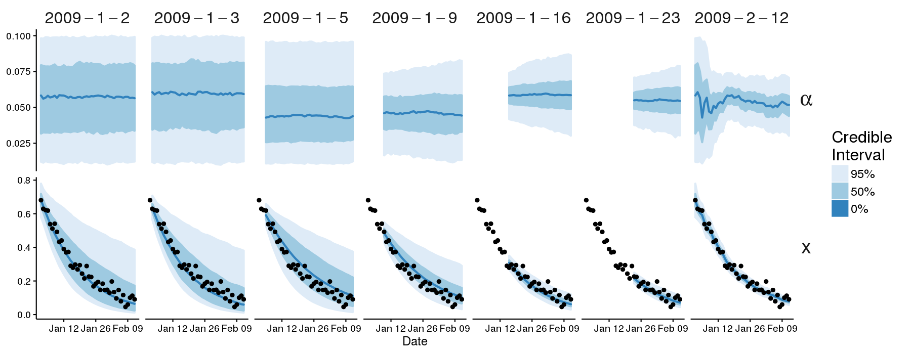
Credible intervals for \(\alpha\) (top row) and \(x\) (bottom row, plotted against the observations), shown for each forecast (identified by date at the top of the plot). Note that the right-most plots (“2009–2–12”) show the credible intervals obtained by using all of the observations.
To generate and plot forecasts that use the post-regularisation particle filter (post-RPF), run the following commands from the root directory of the pypfilt repository:
./doc/example/run.py --regularisation
./doc/example/plot.R
This will generate forecasts (./doc/example/example-rpf.hdf5) and plot the
credible intervals.
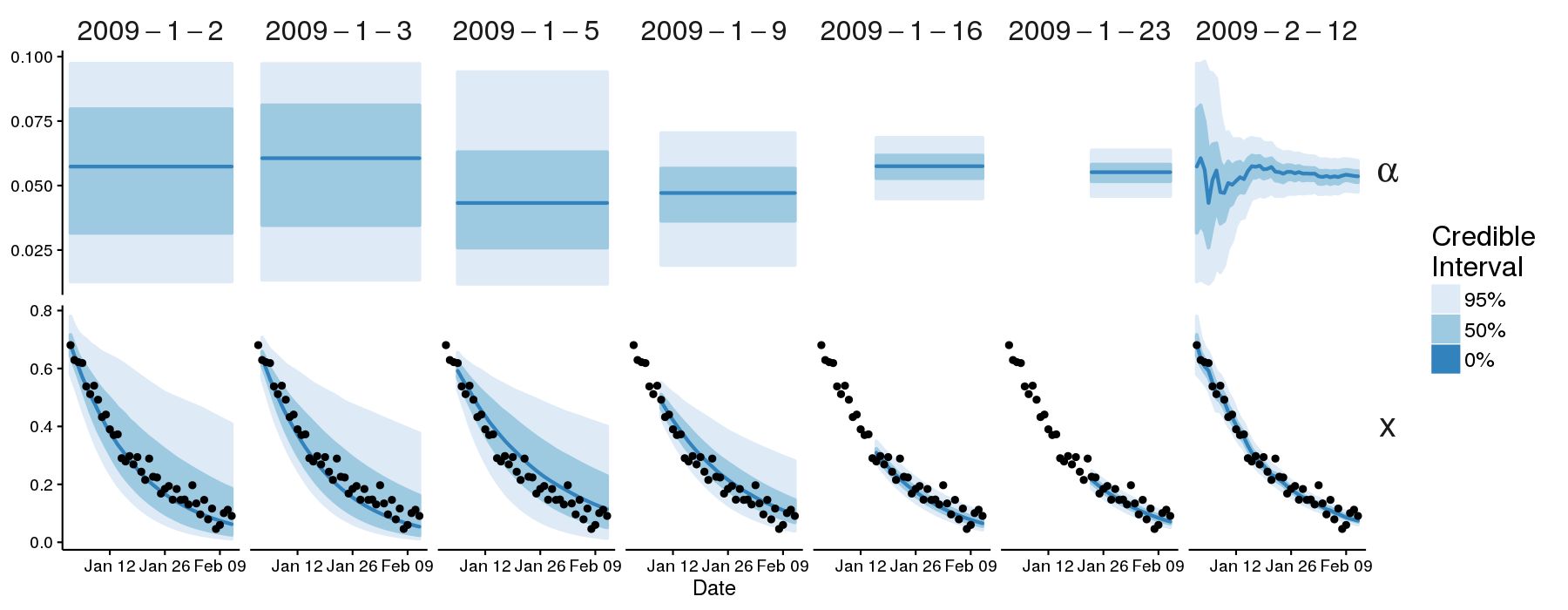
Credible intervals for \(\alpha\) and \(x\) when using the post-regularisation particle filter (post-RPF).