Getting Started
This guide assumes that you have already installed pypfilt:
# Install pypfilt with plotting support.
pip install pypfilt[plot]
See the installation instructions for further details.
Lotka-Volterra (predator-prey) equations
Here we will show how to generate forecasts for the (continuous)
Lotka-Volterra equations, which describe the dynamics of biological systems
in which two species interact (one predator, one prey).
The source code is provided in pypfilt.examples.predation.
-
class
pypfilt.examples.predation.LotkaVolterra¶ An implementation of the (continuous) Lotka-Volterra equations.
\[\begin{split}\frac{dx}{dt} &= \alpha x - \beta xy \\ \frac{dy}{dt} &= \delta xy - \gamma y\end{split}\]Symbol Meaning \(x(t)\) The size of the prey population (1,000s). \(y(t)\) The size of the predator population (1,000s). \(\alpha\) Exponential growth rate in the absence of predators. \(\beta\) The rate at which prey suffer from predation. \(\delta\) The predator growth rate, driven by predation. \(\gamma\) Exponential decay rate of the predator population. All of the state variables and parameters are stored in the particle:
\[\mathbf{x_t} = [x, y, \alpha, \beta, \delta, \gamma]^T\]This class also provides a method for generating noisy observations from a known ground truth:
-
obs(sdev, x0, y0, alpha, beta, gamma, delta, t_max, seed=42)¶ Parameters: - sdev – The standard deviation of the observation error.
- x0 – The initial size of the prey population.
- y0 – The initial size of the predator population.
- alpha – The true value of the model parameter alpha.
- beta – The true value of the model parameter beta.
- gamma – The true value of the model parameter gamma.
- delta – The true value of the model parameter delta.
- t_max – The simulation duration.
- seed – The seed for the observation PRNG.
-
Example outputs
The rest of this “Getting Started” guide will demonstrate how to generate forecasts and produce plots like those shown below.
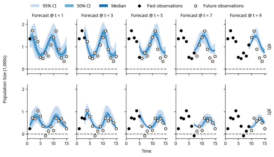
Forecasts produced by the LotkaVolterra model, using noisy
observations generated by this same model (LotkaVolterra.obs())
and a known ground truth.
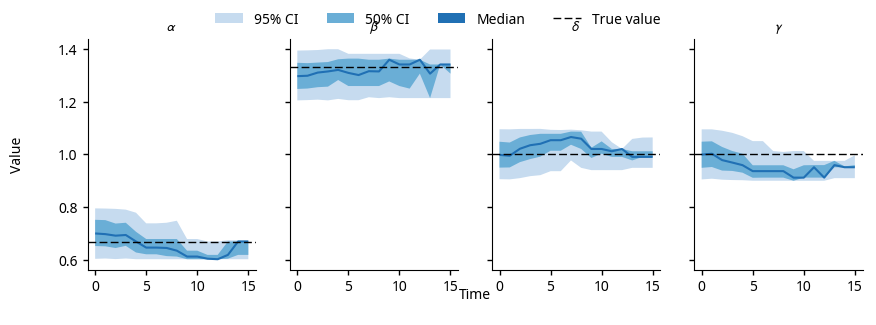
The posterior parameter distributions for the LotkaVolterra
model, using the noisy observations shown in the forecasts above.
Running the forecasts
Model estimations and subsequent forecasts are generated by
pypfilt.forecast(), which takes the following arguments:
- A parameter dictionary, including the system model and the observation model;
- The start and end of the simulation period;
- Any number of observation streams;
- The times at which forecasts should be generated;
- A summary object to calculate relevant statistics; and
- The output file.
One critical parameter is the number of particles to use (px_count).
With too few particles, it is highly likely that none of the particles will be
in good agreement with the observations (“particle degeneracy”).
With too many particles, the computational cost will be very high and the
forecasts will take a long time to complete.
In the example below, 1,000 particles are used (highlighted line).
def forecast(data_file):
    """Run a suite of forecasts against generated observations."""
    logger = logging.getLogger(__name__)
    logger.info('Preparing the forecast simulations')

    # Define the simulation period and forecasting times.
    t0 = 0.0
    t1 = 15.0
    fs_times = [1.0, 3.0, 5.0, 7.0, 9.0]
    params = make_params(px_count=1000, seed=42, obs_sdev=0.2)

    # Generate noisy observations.
    obs = params['model'].obs(params['obs']['sdev'], x0=0.9, y0=0.25,
                              alpha=2/3, beta=4/3, gamma=1, delta=1, t_max=t1)

    # Define the summary tables to be saved to disk.
    summary = pypfilt.summary.HDF5(params, obs, first_day=True)
    summary.add_tables(
        pypfilt.summary.ModelCIs(probs=[0, 50, 95]),
        pypfilt.summary.Obs())

    # Run the forecast simulations.
    pypfilt.forecast(params, t0, t1, [obs], fs_times, summary, data_file)
When generating forecasts on a regular basis (e.g., daily or weekly, in response to new or updated observations) the particle states can be saved to disk to greatly improve the speed with which the forecasts are generated. This is enabled by defining a cache file:
# If the location is not an absolute path, it is defined
# relative to the output directory, params['out_dir'].
params['hist']['cache_file'] = 'cache.hdf5'
Plotting the results
Plotting the forecast results is a two-step process; first, the results must be read from the output file and massaged into the appropriate form, then the plots themselves must be constructed. The first step is illustrated here:
def plot(data_file, png=True, pdf=True):
    logger = logging.getLogger(__name__)
    logger.info('Loading outputs from {}'.format(data_file))

    # Use the 'Agg' backend so that plots can be generated non-interactively.
    import matplotlib
    matplotlib.use('Agg')

    # File names for the generated plots.
    fs_pdf = 'predation_forecasts.pdf'
    fs_png = 'predation_forecasts.png'
    pp_pdf = 'predation_params.pdf'
    pp_png = 'predation_params.png'

    # Read in the model credible intervals and the observations.
    with h5py.File(data_file) as f:
        cints = f['/data/model_cints'][()]
        obs = f['/data/obs'][()]

    # Convert serialised values into more convenient data types.
    convs = pypfilt.summary.default_converters(pypfilt.Scalar())
    cints = pypfilt.summary.convert_cols(cints, convs)
    obs = pypfilt.summary.convert_cols(obs, convs)

    # Separate the observations of the two populations.
    x_obs = obs[obs['unit'] == b'x']
    y_obs = obs[obs['unit'] == b'y']

    # Separate the credible intervals for the population sizes from the
    # credible intervals for the model parameters.
    var_mask = np.logical_or(cints['name'] == b'x',
                             cints['name'] == b'y')
    state_cints = cints[var_mask]
    param_cints = cints[np.logical_not(var_mask)]

    # Only keep the population sizes from each forecast.
    fs_mask = state_cints['fs_date'] < max(state_cints['date'])
    state_cints = state_cints[fs_mask]

    # Only keep the model parameter posteriors from the estimation run.
    est_mask = param_cints['fs_date'] == max(param_cints['date'])
    param_cints = param_cints[est_mask]

    # Plot the population forecasts.
    pdf_file = fs_pdf if pdf else None
    png_file = fs_png if png else None
    plot_forecasts(state_cints, x_obs, y_obs, pdf_file, png_file)

    # Plot the model parameter posterior distributions.
    pdf_file = pp_pdf if pdf else None
    png_file = pp_png if png else None
    plot_params(param_cints, pdf_file, png_file)
The pypfilt.plot module provides functions for plotting observations
and credible intervals, and classes for constructing figures with sub-plots.
These are highlighted in the following two functions, which were used to
produce the figures shown at the top of this guide.
def plot_forecasts(state_cints, x_obs, y_obs, pdf_file=None, png_file=None):
    """Plot the population predictions at each forecasting date."""
    logger = logging.getLogger(__name__)
    with pypfilt.plot.apply_style():
        plot = pypfilt.plot.Grid(
            state_cints, 'Time', 'Population Size (1,000s)',
            ('fs_date', 'Forecast @ t = {:0.0f}'),
            ('name', lambda bs: '{}(t)'.format(pypfilt.text.to_unicode(bs))))
        plot.expand_x_lims('date')
        plot.expand_y_lims('ymax')

        for (ax, df) in plot.subplots():
            ax.axhline(y=0, xmin=0, xmax=1,
                       linewidth=1, linestyle='--', color='k')
            hs = pypfilt.plot.cred_ints(ax, df, 'date', 'prob')
            if df['name'][0] == b'x':
                df_obs = x_obs
            else:
                df_obs = y_obs
            past_obs = df_obs[df_obs['date'] <= df['fs_date'][0]]
            future_obs = df_obs[df_obs['date'] > df['fs_date'][0]]
            hs.extend(pypfilt.plot.observations(ax, past_obs,
                                                label='Past observations'))
            hs.extend(pypfilt.plot.observations(ax, future_obs,
                                                future=True,
                                                label='Future observations'))
            plot.add_to_legend(hs)

            # Adjust the axis limits and the number of ticks.
            ax.set_xlim(left=0)
            ax.locator_params(axis='x', nbins=4)
            ax.set_ylim(bottom=-0.2)
            ax.locator_params(axis='y', nbins=4)

        plot.legend(loc='upper center', ncol=5)

        if pdf_file:
            logger.info('Plotting to {}'.format(pdf_file))
            plot.save(pdf_file, format='pdf', width=10, height=5)
        if png_file:
            logger.info('Plotting to {}'.format(png_file))
            plot.save(png_file, format='png', width=10, height=5)
def plot_params(param_cints, pdf_file=None, png_file=None):
    """Plot the parameter posteriors over the estimation run."""
    logger = logging.getLogger(__name__)
    with pypfilt.plot.apply_style():
        plot = pypfilt.plot.Wrap(
            param_cints, 'Time', 'Value',
            ('name', lambda bs: '$\\{}$'.format(pypfilt.text.to_unicode(bs))),
            nr=1)
        plot.expand_y_lims('ymax')

        for (ax, df) in plot.subplots():
            hs = pypfilt.plot.cred_ints(ax, df, 'date', 'prob')
            if df['name'][0] == b'alpha':
                y_true = 2/3
            elif df['name'][0] == b'beta':
                y_true = 4/3
            elif df['name'][0] == b'gamma':
                y_true = 1
            elif df['name'][0] == b'delta':
                y_true = 1
            hs.append(ax.axhline(y=y_true, xmin=0, xmax=1, label='True value',
                                 linewidth=1, linestyle='--', color='k'))
            plot.add_to_legend(hs)

        plot.legend(loc='upper center', ncol=5)

        if pdf_file:
            logger.info('Plotting to {}'.format(pdf_file))
            plot.save(pdf_file, format='pdf', width=10, height=3)
        if png_file:
            logger.info('Plotting to {}'.format(png_file))
            plot.save(png_file, format='png', width=10, height=3)
Observations
Observations are represented as dictionaries that have the following keys:
{'date': ...,  # When the observation was made (number, date, etc)
 'value': 200,  # The numerical quantity that was measured
 'unit': 'Some measure',  # A description of the measurement units
 'period': 7,  # The observation period, in days
 'source': 'Some system',  # A description of the data source
}
An observation stream is represented as a chronologically sorted list of
observations (oldest first).
The particle filter accepts any number of observation streams, which must be
provided as a list (i.e., a list of observation lists); see
forecast() and run().
Observation models
For simplicity, we assume that both the prey and predator populations — \(x(t)\) and \(y(t)\) — are directly observed, and that the observation error is distributed normally with zero mean and a known standard deviation.
def log_llhd(params, obs_list, curr, prev_dict, weights):
    """Calculate the observation log-likelihoods for each particle."""
    # The expected observations are x(t) and y(t).
    x_dist = scipy.stats.norm(loc=curr[..., 0], scale=params['obs']['sdev'])
    y_dist = scipy.stats.norm(loc=curr[..., 1], scale=params['obs']['sdev'])
    # Calculate the log-likelihood of each observation in turn.
    log_llhd = np.zeros(curr.shape[:-1])
    for o in obs_list:
        if o['unit'] == 'x':
            log_llhd += x_dist.logpdf(o['value'])
        elif o['unit'] == 'y':
            log_llhd += y_dist.logpdf(o['value'])
        else:
            raise ValueError('invalid observation')
    return log_llhd
The observation model must be stored in params['log_llhd_fn'].
Note that the argument prev_dict can be used to obtain the state vectors
at the beginning of an observation period.
This is useful for situations where the observation depends on the change
in the state vector over the observation period.
def log_llhd(params, obs_list, curr, prev_dict, weights):
    # Obtain the state vectors two time units ago.
    # This is only valid if an observation has a period of 2.
    prev_state = prev_dict[2]
    dx = curr[..., 0] - prev_state[..., 0]
    ...
Parameters
Particle filter parameters are provided by default_params().
At a minimum, the simulation parameters must define the model, the time scale,
and the observation model.
For reproducibility, it is also advisable to set the PRNG seed.
def make_params(px_count, seed, obs_sdev):
    """Define the default simulation parameters for this model."""
    model = LotkaVolterra()
    time_scale = pypfilt.Scalar()
    params = pypfilt.default_params(model, time_scale, px_count=px_count)
    # Use one time-step per unit time, odeint will interpolate as needed.
    params['steps_per_unit'] = 1
    params['log_llhd_fn'] = log_llhd
    params['obs'] = {'sdev': obs_sdev}
    # Set the PRNG seed.
    params['resample']['prng_seed'] = seed
    # Write output to the working directory.
    params['out_dir'] = '.'
    params['tmp_dir'] = '.'
    return params
System models
The model of the underlying system must inherit from pypfilt.Model.
Here is the predator-prey model from pypfilt.examples.predation:
class LotkaVolterra(pypfilt.Model):
    """An implementation of the (continuous) Lotka-Volterra equations."""

    def init(self, params, vec):
        """Initialise a matrix of state vectors."""
        # Select x(0), y(0), and the parameters according to the priors.
        rnd = params['resample']['rnd']
        size = vec[..., 0].shape
        vec[..., 0] = params['prior']['x'](rnd, size)
        vec[..., 1] = params['prior']['y'](rnd, size)
        vec[..., 2] = params['prior']['alpha'](rnd, size)
        vec[..., 3] = params['prior']['beta'](rnd, size)
        vec[..., 4] = params['prior']['gamma'](rnd, size)
        vec[..., 5] = params['prior']['delta'](rnd, size)

    def state_size(self):
        """Return the size of the state vector."""
        return 6

    def priors(self, params):
        """Return a dictionary of model priors."""
        return {
            'x': lambda r, size=None: r.uniform(0.5, 1.5, size=size),
            'y': lambda r, size=None: r.uniform(0.2, 0.4, size=size),
            'alpha': lambda r, size=None: r.uniform(0.6, 0.8, size=size),
            'beta': lambda r, size=None: r.uniform(1.2, 1.4, size=size),
            'gamma': lambda r, size=None: r.uniform(0.9, 1.1, size=size),
            'delta': lambda r, size=None: r.uniform(0.9, 1.1, size=size),
        }

    def d_dt(self, xt, t):
        """Calculate the derivatives of x(t) and y(t)."""
        # Restore the 2D shape of the flattened state matrix.
        xt = xt.reshape((-1, 6))
        x, y = xt[..., 0], xt[..., 1]
        d_dt = np.zeros(xt.shape)
        # Calculate dx/dt and dy/dt.
        d_dt[..., 0] = xt[..., 2] * x - xt[..., 3] * x * y
        d_dt[..., 1] = xt[..., 4] * x * y - xt[..., 5] * y
        # Flatten the 2D derivatives matrix.
        return d_dt.reshape(-1)

    def update(self, params, t, dt, is_fs, prev, curr):
        """Perform a single time-step."""
        # Use scalar time, so that ``t + dt`` is well-defined.
        t = params['time'].to_scalar(t)
        # The state matrix must be flattened for odeint.
        xt = scipy.integrate.odeint(self.d_dt, prev.reshape(-1),
                                    [t, t + dt])[1]
        # Restore the 2D shape of the flattened state matrix.
        curr[:] = xt.reshape(curr.shape)

    def describe(self):
        """Describe each component of the state vector."""
        return [
            # Restrict x(t), y(t) to [0, 10^5], don't allow regularisation.
            ('x', False, 0, 1e5),
            ('y', False, 0, 1e5),
            # Restrict parameters to [0, 2], allow regularisation.
            ('alpha', True, 0, 2),
            ('beta', True, 0, 2),
            ('gamma', True, 0, 2),
            ('delta', True, 0, 2),
        ]

    def obs(self, sdev, x0, y0, alpha, beta, gamma, delta, t_max, seed=42):
        """Generate noisy observations from a known ground truth."""
        # Make the priors reflect the known ground truth.
        rnd = np.random.RandomState(seed)
        obs_params = {
            'resample': {
                'rnd': rnd,
            },
            'prior': {
                'x': lambda r, size=None: x0 * np.ones(size),
                'y': lambda r, size=None: y0 * np.ones(size),
                'alpha': lambda r, size=None: alpha * np.ones(size),
                'beta': lambda r, size=None: beta * np.ones(size),
                'gamma': lambda r, size=None: gamma * np.ones(size),
                'delta': lambda r, size=None: delta * np.ones(size),
            },
        }
        # Simulate a single particle.
        xt_init = np.zeros((1, self.state_size()))
        self.init(obs_params, xt_init)
        xt = scipy.integrate.odeint(self.d_dt, xt_init.reshape(-1),
                                    range(int(np.ceil(t_max + 1))))[1:]
        # Observe both populations once per time unit.
        obs = []
        for (ix, x) in enumerate(xt):
            obs.append({'date': ix + 1, 'period': 1, 'unit': 'x',
                        'value': rnd.normal(x[0], sdev),
                        'source': 'noisy_obs()'})
            obs.append({'date': ix + 1, 'period': 1, 'unit': 'y',
                        'value': rnd.normal(x[1], sdev),
                        'source': 'noisy_obs()'})
        return obs
Summary objects
Simulations typically comprise a large number of both particles and time steps, and so it is generally preferable to record statistics that summarise the particles than to store the entire state history of each simulation.
This functionality is provided by pypfilt.summary.HDF5, which allows
any number of summary tables to be recorded. Once all of the estimation and
forecasting simulations have been performed,
save_forecasts() will save the results to disk.
The example shown in Running the forecasts (and repeated below, with the relevant
lines highlighted) demonstrates how to record fixed-probability central
credible intervals for the state variables and model parameters with the
ModelCIs table, and the observations with the
Obs table.
These are the same tables that were used to produce the plots show in
Example outputs.
def forecast(data_file):
    """Run a suite of forecasts against generated observations."""
    logger = logging.getLogger(__name__)
    logger.info('Preparing the forecast simulations')

    # Define the simulation period and forecasting times.
    t0 = 0.0
    t1 = 15.0
    fs_times = [1.0, 3.0, 5.0, 7.0, 9.0]
    params = make_params(px_count=1000, seed=42, obs_sdev=0.2)

    # Generate noisy observations.
    obs = params['model'].obs(params['obs']['sdev'], x0=0.9, y0=0.25,
                              alpha=2/3, beta=4/3, gamma=1, delta=1, t_max=t1)

    # Define the summary tables to be saved to disk.
    summary = pypfilt.summary.HDF5(params, obs, first_day=True)
    summary.add_tables(
        pypfilt.summary.ModelCIs(probs=[0, 50, 95]),
        pypfilt.summary.Obs())

    # Run the forecast simulations.
    pypfilt.forecast(params, t0, t1, [obs], fs_times, summary, data_file)