Forecast performance#
It was visually evident from the previous figures that the post-regularised particle filter produced much better forecasts than the bootstrap particle filter.
However, if there wasn’t such a clear difference between the forecasts, or if we were interested in evaluating forecast performance over a large number of forecasts, visually inspecting the results would not be a suitable approach.
Instead, we can use a proper scoring rule such as the Continuous Ranked Probability Score to evaluate each forecast distribution against the true observations.
We can then measure how much post-regularisation improves the forecast performance by calculating a CRPS skill score relative to the original forecast:
Note
Depending on the nature of the data and your model, it may be useful to transform the data before calculating CRPS values (e.g., computing scores on the log scale). See Scoring epidemiological forecasts on transformed scales (Bosse et al., 2023) for further details.
Shown below are the CPRS values for each \(z(t)\) forecast. As displayed in the figure legend, the forecast with post-regularisation is 76.7% better than the original forecast.
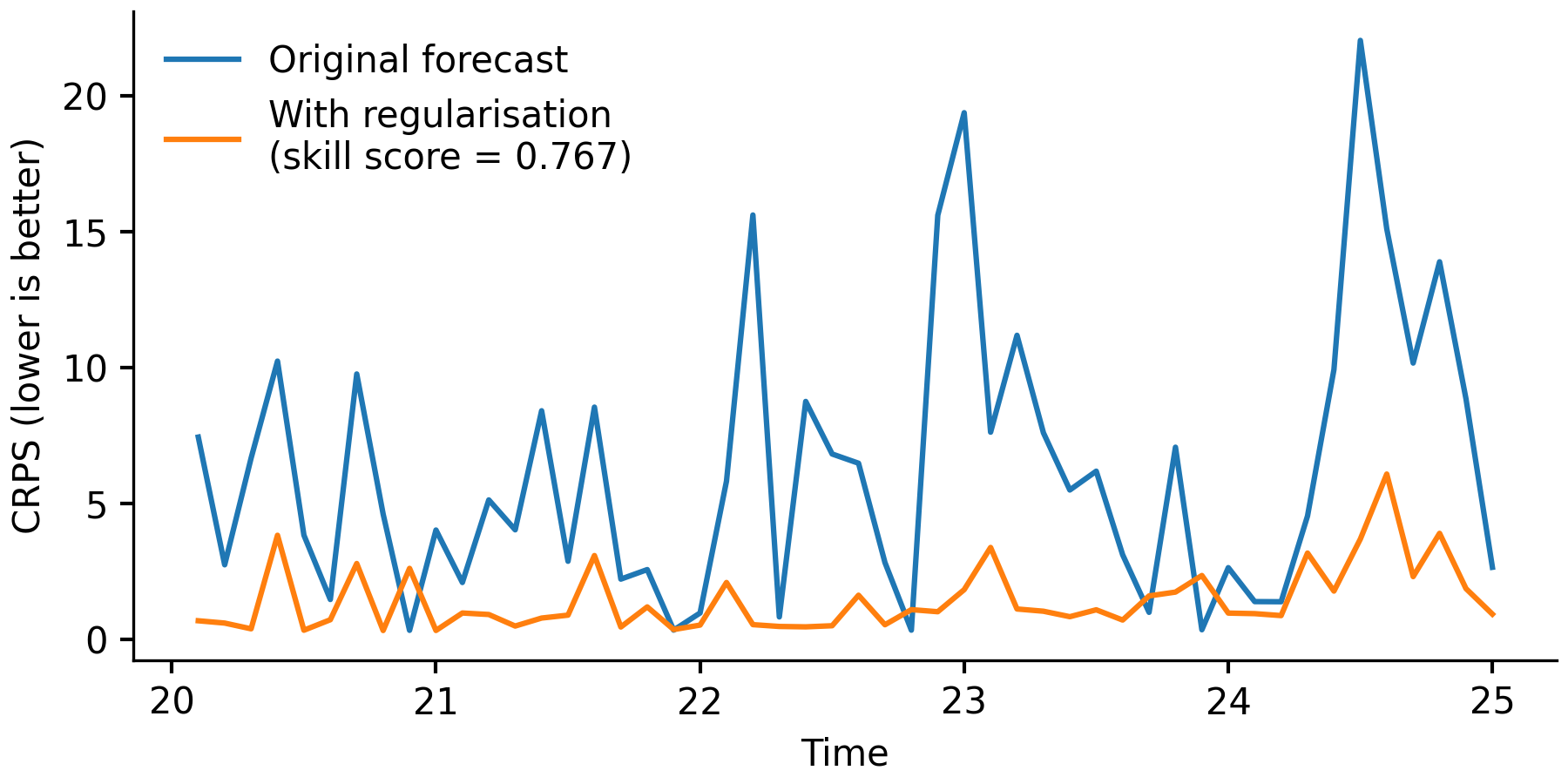
Comparison of CRPS values for the original \(z(t)\) forecasts, and for the \(z(t)\) forecasts with regularisation.#
We can calculate CPRS values by taking the following steps:
Record simulated \(z(t)\) observations for each particle with the
SimulatedObssummary table;Save the forecast results to HDF5 files;
Load the simulated \(z(t)\) observations with
load_summary_table();Load the true future \(z(t)\) observations with
read_table(); andCalculate CRPS values with
simulated_obs_crps().
def score_lorenz63_forecasts():
    """Calculate CRPS values for the simulated `z(t)` observations."""
    # Load the true observations that occur after the forecasting time.
    columns = [('time', float), ('value', float)]
    z_true = pypfilt.io.read_table('lorenz63-z.ssv', columns)
    z_true = z_true[z_true['time'] > 20]

    # Run the original forecasts.
    fs_file = 'lorenz63_forecast.hdf5'
    fs = run_lorenz63_forecast(filename=fs_file)

    # Run the forecasts with regularisation.
    reg_file = 'lorenz63_regularised.hdf5'
    fs_reg = run_lorenz63_forecast_regularised(filename=reg_file)

    # Check that load_observations() returns the expected tables.
    tbl_obs_fs = pypfilt.io.load_observations(fs_file)
    tbl_obs_reg = pypfilt.io.load_observations(reg_file)
    obs_keys = {'x', 'y', 'z'}
    assert obs_keys == set(tbl_obs_fs.keys())
    assert obs_keys == set(tbl_obs_reg.keys())
    for k in obs_keys:
        assert np.array_equal(tbl_obs_fs[k], tbl_obs_reg[k])
        assert len(tbl_obs_fs[k].dtype.fields) == 2
        assert set(tbl_obs_fs[k].dtype.fields.keys()) == {'time', 'value'}

    # Check that load_observations() can return a subset of the observations.
    subset = {'x', 'z'}
    tbl_subset = pypfilt.io.load_observations(reg_file, obs_units=subset)
    assert set(tbl_subset.keys()) == subset

    # Check that load_observations() raises an exception if there are no
    # observations for a given observation unit.
    invalid_subset = {'x', 'zzz'}
    with pytest.raises(
        ValueError, match="Missing observations\\(s\\): \\{'zzz'\\}"
    ):
        pypfilt.io.load_observations(reg_file, obs_units=invalid_subset)

    # Check that load_summary_tables() returns the expected tables.
    tbl_sum_fs = pypfilt.io.load_summary_tables(fs_file)
    tbl_sum_reg = pypfilt.io.load_summary_tables(reg_file)
    tbl_keys = {'forecasts', 'sim_z'}
    assert tbl_keys == set(tbl_sum_fs.keys())
    assert tbl_keys == set(tbl_sum_reg.keys())
    for k in tbl_keys:
        # We should have identical data types, but different results.
        assert tbl_sum_fs[k].dtype == tbl_sum_reg[k].dtype
        assert not np.array_equal(tbl_sum_fs[k], tbl_sum_reg[k])

    # Check that load_summary_tables() can return a subset of the tables.
    subset = {'forecasts'}
    tbl_subset = pypfilt.io.load_summary_tables(reg_file, table_names=subset)
    assert set(tbl_subset.keys()) == subset

    # Check that load_summary_tables() raises an exception if a named table
    # doesn't exist.
    invalid_subset = {'forecasts', 'something_missing'}
    with pytest.raises(
        ValueError, match="Missing table\\(s\\): \\{'something_missing'\\}"
    ):
        pypfilt.io.load_summary_tables(reg_file, table_names=invalid_subset)

    # Extract the simulated z(t) observations for each forecast.
    time = pypfilt.Scalar()
    z_table = '/tables/sim_z'
    z_fs = pypfilt.io.load_summary_table(time, fs_file, z_table)
    z_reg = pypfilt.io.load_summary_table(time, reg_file, z_table)

    # Calculate CRPS values for each forecast.
    crps_fs = pypfilt.crps.simulated_obs_crps(z_true, z_fs)
    crps_reg = pypfilt.crps.simulated_obs_crps(z_true, z_reg)

    # Check that regularisation improved the forecast performance.
    assert np.mean(crps_reg['score']) < np.mean(crps_fs['score'])

    # Compare the CRPS values for each forecast.
    plot_crps_comparison(crps_fs, crps_reg, 'lorenz63_crps_comparison.png')

    return (fs, fs_reg)