Regularisation

We can maintain particle diversity with the post-regularised particle filter, where resampling draws particles from a continuous distribution, rather than directly from the particle ensemble. The continuous distribution is constructed using a multi-variate Gaussian kernel, whose covariance matrix is the normalised particle covariance. This means that when the particles are resampled, we will obtain many particles that are similar, but not identical to the particles with the largest weights (i.e., those that best describe the past observations).

As demonstrated in the figure below, the post-regularised particle filter greatly improves the model fit and forecasts. However, due to the chaotic nature of the system, the forecasts for \(x(t)\) and \(y(t)\) become quite uncertain by \(t=25\).

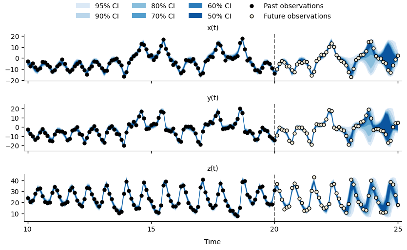
Forecasts for \(x(t)\), \(y(t)\), and \(z(t)\) of the Lorenz63 system at time \(t=20\), using the post-regularisation particle filter.

In order to use the post-regularised particle filter, we need to:

1. Identify which fields in the particle state vector can be smoothed by the filter. This is defined by the simulation model’s can_smooth() method.

2. Enable regularisation by setting filter.regularisation.enabled = true in the scenario definition.

3. Define the lower and upper bounds for each field that should be smoothed (filter.regularisation.bounds.FIELD) in the scenario definition.

Note

The post-regularised particle filter will only smooth fields that are returned by the can_smooth() method and for which lower and/or upper bounds have been defined.

You can omit the lower or upper bounds, if they are not appropriate. To smooth a field without imposing any bounds, define an empty table for that field. See the bounds for z in the scenario definition below.

The Lorenz63 simulation model allows all state vector fields to be smoothed (see highlighted lines).

class Lorenz63(OdeModel):
    def field_types(self, ctx):
        r"""
        Define the state vector :math:`[\sigma, \rho, \beta, x, y, z]^T`.
        """
        return [
            ('sigma', float),
            ('rho', float),
            ('beta', float),
            ('x', float),
            ('y', float),
            ('z', float),
        ]

    def d_dt(self, time, xt, ctx, is_forecast):
        """
        The right-hand side of the ODE system.

        :param time: The current time.
        :param xt: The particle state vectors.
        :param ctx: The simulation context.
        :param is_forecast: True if this is a forecasting simulation.
        """
        rates = np.zeros(xt.shape, xt.dtype)
        rates['x'] = xt['sigma'] * (xt['y'] - xt['x'])
        rates['y'] = xt['x'] * (xt['rho'] - xt['z']) - xt['y']
        rates['z'] = xt['x'] * xt['y'] - xt['beta'] * xt['z']
        return rates

    def can_smooth(self):
        """Indicate which state vector fields can be smoothed."""
        return {'sigma', 'rho', 'beta', 'x', 'y', 'z'}

An example scenario for the Lorenz-63 system that uses the post-regularisation particle filter (see highlighted lines).

# NOTE: Save this file as 'lorenz63_forecast_regularised.toml'

[components]
model = "pypfilt.examples.lorenz.Lorenz63"
time = "pypfilt.Scalar"
sampler = "pypfilt.sampler.LatinHypercube"
summary = "pypfilt.summary.HDF5"

[time]
start = 0.0
until = 25.0
steps_per_unit = 10
summaries_per_unit = 10

[prior]
sigma = { name = "constant", args.value = 10 }
rho = { name = "constant", args.value = 28 }
beta = { name = "constant", args.value = 2.66667 }
x = { name = "uniform", args.loc = -5, args.scale = 10 }
y = { name = "uniform", args.loc = -5, args.scale = 10 }
z = { name = "uniform", args.loc = -5, args.scale = 10 }

[summary.tables]
forecasts.component = "pypfilt.summary.PredictiveCIs"
forecasts.credible_intervals = [50, 60, 70, 80, 90, 95]
sim_z.component = "pypfilt.summary.SimulatedObs"
sim_z.observation_unit = "z"

[observations.x]
model = "pypfilt.examples.lorenz.ObsLorenz63"
file = "lorenz63-x.ssv"

[observations.y]
model = "pypfilt.examples.lorenz.ObsLorenz63"
file = "lorenz63-y.ssv"

[observations.z]
model = "pypfilt.examples.lorenz.ObsLorenz63"
file = "lorenz63-z.ssv"

[filter]
particles = 500
prng_seed = 2001
history_window = -1
resample.threshold = 0.25
regularisation.enabled = true

[filter.regularisation.bounds]
x = { min = -50, max = 50 }
y = { min = -50, max = 50 }
z = {}

[scenario.forecast_regularised]

Note

Call save_lorenz63_scenario_files() to save this scenario file (and the others used in this tutorial) in the working directory.

def run_lorenz63_forecast_regularised(filename=None):
    scenario_file = 'lorenz63_forecast_regularised.toml'
    instances = list(pypfilt.load_instances(scenario_file))
    instance = instances[0]

    # Run a forecast from t = 20.
    forecast_time = 20
    context = instance.build_context()
    return pypfilt.forecast(context, [forecast_time], filename=filename)